Curve that touches three points: Difference between revisions

Content added Content deleted

Inline

Revision as of 20:31, 10 June 2022

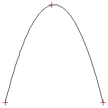
Draw a curve that touches 3 points (1 starting point, 2 medium, 3 final point)

Do not use functions of a library, implement the curve() function yourself
coordinates:(x,y) starting point (10,10) medium point (100,200) final point (200,10)

Action!

Library: Action! Tool Kit

Library: Action! Real Math

<lang Action!>INCLUDE "H6:REALMATH.ACT"

TYPE Point=[INT x,y]

PROC QuadraticCurve(Point POINTER p1,p2,p3 REAL POINTER a,b,c)

 REAL x1,y1,x2,y2,x3,y3,x11,x22,x33,m,n,tmp1,tmp2,tmp3,tmp4,r1

 IntToRealForNeg(-1,r1)
 IntToRealForNeg(p1.x,x1) IntToRealForNeg(p1.y,y1)
 IntToRealForNeg(p2.x,x2) IntToRealForNeg(p2.y,y2)
 IntToRealForNeg(p3.x,x3) IntToRealForNeg(p3.y,y3)

 RealMult(x1,x1,x11) ;x11=x1^2
 RealMult(x2,x2,x22) ;x22=x2^2
 RealMult(x3,x3,x33) ;x33=x3^2

 RealSub(x1,x2,m)   ;m=x1-x2
 RealSub(x3,x2,n)   ;n=x3-x2
 RealMult(m,n,tmp1) ;tmp1=m*n

 IF IsNegative(tmp1) THEN
   RealMult(m,r1,tmp1)
   RealAssign(tmp1,m)  ;m=-m
 FI

 RealSub(y1,y2,tmp1)     ;tmp1=y1-y2
 RealMult(n,tmp1,tmp2)   ;tmp2=n*(y1-y2)
 RealSub(y3,y2,tmp1)     ;tmp1=y3-y2
 RealMult(m,tmp1,tmp3)   ;tmp3=m*(y3-y2)
 RealAdd(tmp2,tmp3,tmp1) ;tmp1=n*(y1-y2)+m*(y3-y2)

 RealSub(x11,x22,tmp2)   ;tmp2=x1^2-x2^2
 RealMult(n,tmp2,tmp3)   ;tmp3=n*(x1^2-x2^2)
 RealSub(x33,x22,tmp2)   ;tmp2=x3^2-x2^2
 RealMult(m,tmp2,tmp4)   ;tmp4=m*(x3^2-x2^2)
 RealAdd(tmp3,tmp4,tmp2) ;tmp2=n*(x1^2-x2^2)+m*(x3^2-x2^2)

 RealDiv(tmp1,tmp2,a)    ;a=(n*(y1-y2)+m*(y3-y2)) / (n*(x1^2-x2^2)+m*(x3^2-x2^2))

 RealSub(x33,x22,tmp1)   ;tmp1=x3^2-x2^2
 RealMult(tmp1,a,tmp2)   ;tmp2=(x3^2-x2^2)*a
 RealSub(y3,y2,tmp1)     ;tmp1=y3-y2
 RealSub(tmp1,tmp2,tmp3) ;tmp3=(y3-y2)-(x3^2-x2^2)*a
 
 RealSub(x3,x2,tmp1)     ;tmp1=x3-x2
 RealDiv(tmp3,tmp1,b)    ;b=((y3-y2)-(x3^2-x2^2)*a) / (x3-x2)

 RealMult(a,x11,tmp1)    ;tmp1=a*x1^2
 RealMult(b,x1,tmp2)     ;tmp2=b*x1
 RealSub(y1,tmp1,tmp3)   ;tmp3=y1-a*x1^2
 RealSub(tmp3,tmp2,c)    ;c=y1-a*x1^2-b*x1

RETURN

PROC DrawPoint(INT x,y)

 Plot(x-2,y-2) DrawTo(x+2,y-2)
 DrawTo(x+2,y+2) DrawTo(x-2,y+2)
 DrawTo(x-2,y-2)

RETURN

INT FUNC Min(INT a,b)

 IF ab THEN RETURN (a) FI

RETURN (b)
INT FUNC CalcY(REAL POINTER a,b,c INT xi)
REAL xr,xr2,yr,tmp1,tmp2,tmp3 INT yi
IntToRealForNeg(xi,xr) ;xr=x RealMult(xr,xr,xr2) ;xr2=x^2 RealMult(a,xr2,tmp1) ;tmp1=a*x^2 RealMult(b,xr,tmp2) ;tmp2=b*x RealAdd(tmp1,tmp2,tmp3) ;tmp3=a*x^2+b*x RealAdd(tmp3,c,yr) ;y3=a*x^2+b*x+c yi=Round(yr)
RETURN (yi)
PROC DrawCurve(Point POINTER p1,p2,p3)
REAL a,b,c INT xi,yi,minX,maxX
QuadraticCurve(p1,p2,p3,a,b,c)
DrawPoint(p1.x,p1.y) DrawPoint(p2.x,p2.y) DrawPoint(p3.x,p3.y)
minX=Min(p1.x,p2.x) minX=Min(minX,p3.x) maxX=Max(p1.x,p2.x) maxX=Max(maxX,p3.x)
yi=CalcY(a,b,c,minX) Plot(minX,yi) FOR xi=minX TO maxX DO yi=CalcY(a,b,c,xi) DrawTo(xi,yi) OD
RETURN
PROC Main()
BYTE CH=$02FC,COLOR1=$02C5,COLOR2=$02C6 Point p1,p2,p3
Graphics(8+16) Color=1 COLOR1=$0C COLOR2=$02
p1.x=10 p1.y=10 p2.x=100 p2.y=180 p3.x=200 p3.y=10 DrawCurve(p1,p2,p3)
DO UNTIL CH#$FF OD CH=$FF
RETURN</lang>

Output:
Screenshot from Atari 8-bit computer
Ada
Find center and radius of circle that touches the 3 points. Solve with simple linear algebra. In this case no division by zero. <lang Ada>with Ada.Text_Io; with Ada.Numerics.Generic_Elementary_Functions;
procedure Three_Point_Circle is
type Real is new Float;
package Real_Math is new Ada.Numerics.Generic_Elementary_Functions (Real);
package Real_Io is new Ada.Text_Io.Float_Io (Real);
use Real_Io, Ada.Text_Io;
-- Point P1 X1 : constant Real := 10.0; Y1 : constant Real := 10.0;
-- Point P2 X2 : constant Real := 100.0; Y2 : constant Real := 200.0;
-- Point P3 X3 : constant Real := 200.0; Y3 : constant Real := 10.0;
-- Point P4 - midpoint between P1 and P2 X4 : constant Real := (X1 + X2) / 2.0; Y4 : constant Real := (Y1 + Y2) / 2.0; S4 : constant Real := (Y2 - Y1) / (X2 - X1); -- Slope P1-P2 A4 : constant Real := -1.0 / S4; -- Slope P4-Center -- Y4 = A4 * X4 + B4 <=> B4 = Y4 - A4 * X4 B4 : constant Real := Y4 - A4 * X4;
-- Point P5 - midpoint between P2 and P3 X5 : constant Real := (X2 + X3) / 2.0; Y5 : constant Real := (Y2 + Y3) / 2.0; S5 : constant Real := (Y3 - Y2) / (X3 - X2); -- Slope P2-P3 A5 : constant Real := -1.0 / S5; -- Slope P5-Center -- Y5 = A5 * X5 + B5 <=> B5 = Y5 - A5 * X5 B5 : constant Real := Y5 - A5 * X5;
-- Find center -- Y = A4 * X + B4 -- Line 1 -- Y = A5 * X + B5 -- Line 2 -- Solve for X: -- A4 * X + B4 = A5 * X + B5 -- A4 * X - A5 * X = B5 - B4 -- X * (A4 - A5) = B5 - B4 -- X = (B5 - B4) / (A4 - A5) Xc : constant Real := (B5 - B4) / (A4 - A5); Yc : constant Real := A4 * Xc + B4; -- Radius R : constant Real := Real_Math.Sqrt ((X1 - Xc) ** 2 + (Y1 - Yc) ** 2);
begin
Real_Io.Default_Exp := 0; Real_Io.Default_Aft := 1;
Put ("Center : "); Put ("("); Put (Xc); Put (", "); Put (Yc); Put (")"); New_Line; Put ("Radius : "); Put (R); New_Line;
end Three_Point_Circle;</lang>

Output:
Center : (105.0, 81.3) Radius : 118.8
AutoHotkey
<lang AutoHotkey>QuadraticCurve(p1,p2,p3){ ; Y = aX^2 + bX + c x1:=p1.1, y1:=p1.2, x2:=p2.1, y2:=p2.2, x3:=p3.1, y3:=p3.2 m:=x1-x2, n:=x3-x2, m:= ((m*n)<0?-1:1) * m a:=(n*(y1-y2)+m*(y3-y2)) / (n*(x1**2 - x2**2) + m*(x3**2 - x2**2)) b:=((y3-y2) - (x3**2 - x2**2)*a) / (x3-x2) c:=y1 - a*x1**2 - b*x1 return [a,b,c] }</lang> Examples:<lang AutoHotkey>P1 := [10,10], P2 := [100,200], P3 := [200,10] v := QuadraticCurve(p1,p2,p3) a := v.1, b:= v.2, c:= v.3 for i, X in [10,100,200]{ Y := a*X**2 + b*X + c ; Y = aX^2 + bX + c res .= "[" x ", " y "]`n" } MsgBox % "Y = " a " X^2 " (b>0?"+":"") b " X " (c>0?"+":"") c " `n" res</lang>
for plotting, use code from RosettaCode: Plot Coordinate Pairs

Outputs:

Y = -0.021111 X^2 +4.433333 X -32.222222 [10, 10.000000] [100, 200.000000] [200, 10.000000]
Go
Library: Go Graphics

There are, of course, an infinity of curves which can be fitted to 3 points. The most obvious solution is to fit a quadratic curve (using Lagrange interpolation) and so that's what we do here.
As we're not allowed to use library functions to draw the curve, we instead divide the x-axis of the curve between successive points into equal segments and then join the resulting points with straight lines.
The resulting 'curve' is then saved to a .png file where it can be viewed with a utility such as EOG. <lang go>package main
import "github.com/fogleman/gg"
var p = [3]gg.Point{{10, 10}, {100, 200}, {200, 10}}
func lagrange(x float64) float64 {
return (x-p[1].X)*(x-p[2].X)/(p[0].X-p[1].X)/(p[0].X-p[2].X)*p[0].Y + (x-p[0].X)*(x-p[2].X)/(p[1].X-p[0].X)/(p[1].X-p[2].X)*p[1].Y + (x-p[0].X)*(x-p[1].X)/(p[2].X-p[0].X)/(p[2].X-p[1].X)*p[2].Y
}
func getPoints(n int) []gg.Point {
pts := make([]gg.Point, 2*n+1) dx := (p[1].X - p[0].X) / float64(n) for i := 0; i < n; i++ { x := p[0].X + dx*float64(i) pts[i] = gg.Point{x, lagrange(x)} } dx = (p[2].X - p[1].X) / float64(n) for i := n; i < 2*n+1; i++ { x := p[1].X + dx*float64(i-n) pts[i] = gg.Point{x, lagrange(x)} } return pts
}
func main() {
const n = 50 // more than enough for this dc := gg.NewContext(210, 210) dc.SetRGB(1, 1, 1) // White background dc.Clear() for _, pt := range getPoints(n) { dc.LineTo(pt.X, pt.Y) } dc.SetRGB(0, 0, 0) // Black curve dc.SetLineWidth(1) dc.Stroke() dc.SavePNG("quadratic_curve.png")
}</lang>
J
NB. coordinates:(x,y) starting point (10,10) medium point (100,200) final point (200,10) X=: 10 100 200 Y=: 10 200 10 NB. matrix division computes polynomial coefficients NB. %. implements singular value decomposition NB. in other words, we can also get best fit polynomials of lower order. polynomial=: (Y %. (^/ ([: i. #)) X)&p. assert 10 200 10 -: polynomial X NB. test Filter=: (#~`)(`:6) Round=: adverb def '<.@:(1r2&+)&.:(%&m)' assert 100 120 -: 100 8 Round 123 NB. test, round 123 to nearest multiple of 100 and of 8 NB. libraries not permitted, character cell graphics are used. GRAPH=: 50 50 $ ' ' NB. is an array of spaces NB. place the axes GRAPH=: '-' [`(([:<0; i.@:#)@:])`]} GRAPH GRAPH=: '|' [`(([:<0;~i.@:#)@:])`]} GRAPH GRAPH=: '+' [`((<0;0)"_)`]} GRAPH NB. origin NB. clip the domain. EXES=: ((<:&(>./X) *. (<./X)&<:))Filter 5 * i. 200 WHYS=: polynomial EXES NB. draw the curve 1j1 #"1 |. 'X' [`((<"1 WHYS ;&>&:([: 1 Round %&5) EXES)"_)`]} GRAPH NB. were we to use a library: load'plot' 'title 3 point fit' plot (j. polynomial) i.201
Julia
To make things more specific, find the circle determined by the points. The curve is then the arc between the 3 points. <lang julia>using Makie
struct Point; x::Float64; y::Float64; end
Find a circle passing through the 3 points
const p1 = Point(10, 10) const p2 = Point(100, 200) const p3 = Point(200, 10) const allp = [p1, p2, p3]
set up problem matrix and solve.

if (x - a)^2 + (y - b)^2 = r^2 then for some D, E, F, x^2 + y^2 + Dx + Ey + F = 0

therefore Dx + Ey + F = -x^2 - y^2
v = zeros(Int, 3) m = zeros(Int, 3, 3) for row in 1:3
m[row, 1:3] .= [allp[row].x, allp[row].y, 1] v[row] = -(allp[row].x)^2 - (allp[row].y)^2
end q = (m \ v) # [-210.0, -162.632, 3526.32] a, b, r = -q[1] / 2, -q[2] / 2, sqrt((q[1]^2/4) + q[2]^2/4 - q[3])
println("The circle with center at x = $a, y = $b and radius $r.")
x = a-r:0.25:a+r y0 = sqrt.(r^2 .- (x .- a).^2) scene = lines(x, y0 .+ b, color = :red) lines!(scene, x, b .- y0, color = :red) scatter!(scene, [p.x for p in allp], [p.y for p in allp], markersize = r / 10)

</lang>

Output:
The circle with center at x = 105.0, y = 81.31578947368422 and radius 118.78948534384199.
Lambdatalk
We find a curve interpolating three points using a bezier algorithm. A bezier curve built on 3 points, p0, p1, p2 doesn't interpolate p1. We compute a new point q symetric of the middle of p0, p2 with respect to p1. The curve built on p0, q, p2 interpolates p0, p1, p2.
bezier interpolation of 3 points
<lang Scheme> p(t) = 1*p0(1-t)2 + 2*p1(1-t)t + 1*p2t2
{def interpol
{lambda {:p0 :p1 :p2 :t :u} // u =1-t {+ {* 1 {A.get 0 :p0} :u :u} {* 2 {A.get 0 :p1} :u :t} {* 1 {A.get 0 :p2} :t :t}} {+ {* 1 {A.get 1 :p0} :u :u} {* 2 {A.get 1 :p1} :u :t} {* 1 {A.get 1 :p2} :t :t}} }}
-> interpol </lang>
two useful functions
<lang Scheme> {def middle
{lambda {:p1 :p2} // compute the middle point of p1 and p2 {A.new {/ {+ {A.get 0 :p1} {A.get 0 :p2}} 2} {/ {+ {A.get 1 :p1} {A.get 1 :p2}} 2} }}}
-> middle
{def symetric // compute the symmetric point of p1 with respect to p2
{lambda {:p1 :p2} {A.new {- {* 2 {A.get 0 :p2}} {A.get 0 :p1} } {- {* 2 {A.get 1 :p2}} {A.get 1 :p1} } }}}
-> symetric </lang>
computing the curve
<lang Scheme> {def curve
{lambda {:pol :n} {S.map {{lambda {:p0 :p1 :p2 :n :i} {interpol :p0 :p1 :p2 {/ :i :n} {- 1 {/ :i :n}}} } {A.get 0 :pol} {A.get 1 :pol} {A.get 2 :pol} :n} {S.serie -1 {+ :n 1}} }}}
-> curve </lang>
drawing a point
<lang Scheme> {def dot
{lambda {:pt} {circle {@ cx="{A.get 0 :pt}" cy="{A.get 1 :pt}" r="5" stroke="#0ff" fill="transparent" stroke-width="2"}}}}
-> dot </lang>
defining points
<lang Scheme> {def P0 {A.new 150 180}} -> P0 {def P1 {A.new 300 250}} -> P1 {def P2 {A.new 150 330}} -> P2
{def P02 {middle {P0} {P2}}} -> P02 {def P20 {symetric {P02} {P1}}} -> P20
{def P10 {middle {P1} {P0}}} -> P10 {def P01 {symetric {P10} {P2}}} -> P01
{def P21 {middle {P2} {P1}}} -> P21 {def P12 {symetric {P21} {P0}}} -> P12 </lang>
drawing points and curves
<lang Scheme> {svg {@ width="500" height="500" style="background:#444;"}
{polyline {@ points="{curve {A.new {P0} {P20} {P2}} 20}" stroke="#f00" fill="transparent" stroke-width="4"}} {polyline {@ points="{curve {A.new {P1} {P01} {P0}} 20}" stroke="#0f0" fill="transparent" stroke-width="4"}} {polyline {@ points="{curve {A.new {P2} {P12} {P1}} 20}" stroke="#00f" fill="transparent" stroke-width="4"}}
{dot {P0}} {dot {P1}} {dot {P2}}
{dot {P02}} {dot {P20}} {dot {P10}} {dot {P01}} {dot {P21}} {dot {P12}}
} </lang>
See the result in http://lambdaway.free.fr/lambdawalks/?view=bezier_3

Mathematica/Wolfram Language
Built-in
<lang Mathematica>pts = {{10, 10}, {100, 200}, {200, 10}}; cs = Circumsphere[pts] Graphics[{PointSize[Large], Point[pts], cs}]</lang>

Output:
Outputs the circle:
Sphere[{105, 1545/19}, (5 Sqrt[203762])/19]
and a graphical representation of the input points and the circle.
Alternate implementation
<lang Mathematica>pts = {{10, 10}, {100, 200}, {200, 10}}; createCircle[{{x1_, y1_}, {x2_, y2_}, {x3_, y3_}}] :=
With[{a = Det[({{x1, y1, 1}, {x2, y2, 1}, {x3, y3, 1}})], d = -Det[({{x1^2 + y1^2, y1, 1}, {x2^2 + y2^2, y2, 1}, {x3^2 + y3^2, y3, 1}})], e = Det[({{x1^2 + y1^2, x1, 1}, {x2^2 + y2^2, x2, 1}, {x3^2 + y3^2, x3, 1}})], f = -Det[({{x1^2 + y1^2, x1, y1}, {x2^2 + y2^2, x2, y2}, {x3^2 + y3^2, x3, y3}})]}, Circle[{-(d/(2 a)), -(e/(2 a))}, Sqrt[(d^2 + e^2)/(4 a^2) - f/a]]]
cs = createCircle[pts] Graphics[{PointSize[Large], Point[pts], cs}]</lang>

Output:
Outputs the circle:
Circle[{105, 1545/19}, (5 Sqrt[203762])/19]
and a graphical representation of the input points and the circle.
Nim
Translation of: Go
Library: imageman
<lang Nim>import imageman
type
FPoint = tuple[x, y: float] FPoints3 = array[3, FPoint]
func lagrange(p: FPoints3; x: float): float =
(x-p[1].x) * (x-p[2].x) / (p[0].x-p[1].x) / (p[0].x-p[2].x) * p[0].y + (x-p[0].x) * (x-p[2].x) / (p[1].x-p[0].x) / (p[1].x-p[2].x) * p[1].y + (x-p[0].x) * (x-p[1].x) / (p[2].x-p[0].x) / (p[2].x-p[1].x) * p[2].y
func points(p: FPoints3; n: int): seq[Point] =
result.setLen(2 * n + 1) var dx = (p[1].x - p[0].x) / float(n) for i in 0..<n: let x = p[0].x + dx * float(i) result[i] = (x.toInt, p.lagrange(x).toInt) dx = (p[2].x - p[1].x) / float(n) for i in n..2*n: let x = p[1].x + dx * float(i - n) result[i] = (x.toInt, p.lagrange(x).toInt)
const N = 50
const P: FPoints3 =[(10.0, 10.0), (100.0, 200.0), (200.0, 10.0)]
var img = initImage[ColorRGBF](210, 210) img.fill(ColorRGBF([float32 1, 1, 1])) # White background. let color = ColorRGBF([float32 0, 0, 0]) # Black. img.drawPolyline(closed = false, color, P.points(N)) img.savePNG("curve.png", compression = 9)</lang>
ooRexx
<lang oorexx>/* REXX ***************************************************************
Compute the polynome satisfying three giveb Points
/
pl='(10,10) (100,200) (200,10)' Do i=1 To 3
Parse Var pl '(' x.i ',' y.i ')' pl s.i=x.i**2 x.i 1 y.i End
Parse Value lingl() With a b c If a<>0 Then
gl=a'*x**2'
Else
gl=
If b>0 & gl<> Then b='+'||b If b<>0 Then gl=gl||b'*x' If c>0 & gl<> Then c='+'||c If c<>0 Then gl=gl||c Say 'y='gl Say 'x / f(x) / y' Do i=1 To 3
Say x.i '/' fun(x.i) '/' y.i End
Exit
fun: Parse Arg x Return a*x**2+b*x+c
lingl: Procedure Expose s. /************************************************* Version: 25.11.1996 *
Lösung eines linearen Gleichungssystems

22.11.1996 PA neu
/
Numeric Digits 12
Do i=1 to 3 l=s.i Do j=1 By 1 While l<> Parse Var l a.1.i.j l End m=j-1 End n=i-1 Do i=1 To n s= Do j=1 To m s=s format(a.1.i.j,6,2) End Call dbg s End
Do ie=1 To i-1
u=ie v=ie+1 Do kk=ie To n If a.u.kk.ie<>0 Then Leave End Select When kk=ie Then Nop When kk>n Then Call ex 'eine Katastrophe' Otherwise Do Do jj=1 To m temp=a.u.ie.jj a.u.ie.jj=a.u.kk.jj a.u.kk.jj=temp End Do ip=1 To n s= Do jp=1 To m s=s format(a.u.ip.jp,12,2) End Call dbg s End End End
Do i=1 To n Do j=1 To m If i<=ie Then a.v.i.j=a.u.i.j Else a.v.i.j=a.u.i.j*a.u.ie.ie-a.u.i.ie*a.u.ie.j End End
Call dbg copies('-',70) Do i=1 To n Do j=1 To m If a.v.i.j<>0 Then Leave End Select When j=m Then Call ex 'Widersprüchliches Gleichungssystem' When j>m Then Call ex 'Gleichungen sind linear abhängig' Otherwise Nop End End Do i=1 To n s= Do j=1 To m s=s format(a.v.i.j,12,2) End Call dbg s End End
n1=n+1 Do i=n To 1 By -1
i1=i+1 x.i=a.v.i.n1/a.v.i.i sub=0 Do j=i+1 To n sub=sub+a.v.i.j*x.j End x.i=x.i-sub/a.v.i.i End
sol= Do i=1 To n sol=sol x.i End
Return sol
ex:
Say arg(1) Exit
dbg: Return</lang>

Output:
y=-0.021111111111*x**2+4.43333333333*x-32.2222222222 x / f(x) / y 10 / 10.0000000 / 10 100 / 200.000000 / 200 200 / 10.0000008 / 10
Perl
Hilbert curve task code repeated here, with the addition that the 3 task-required points are marked. Mostly satisfies the letter-of-the-law of task specification while (all in good fun) subverting the spirit of the thing. <lang perl>use SVG; use List::Util qw(max min);
use constant pi => 2 * atan2(1, 0);
Compute the curve with a Lindemayer-system
%rules = (
A => '-BF+AFA+FB-', B => '+AF-BFB-FA+'
); $hilbert = 'A'; $hilbert =~ s/([AB])/$rules{$1}/eg for 1..6;
Draw the curve in SVG
($x, $y) = (0, 0); $theta = pi/2; $r = 5;
for (split //, $hilbert) {
if (/F/) { push @X, sprintf "%.0f", $x; push @Y, sprintf "%.0f", $y; $x += $r * cos($theta); $y += $r * sin($theta); } elsif (/\+/) { $theta += pi/2; } elsif (/\-/) { $theta -= pi/2; }
}
$max = max(@X,@Y); $xt = -min(@X)+10; $yt = -min(@Y)+10; $svg = SVG->new(width=>$max+20, height=>$max+20); $points = $svg->get_path(x=>\@X, y=>\@Y, -type=>'polyline'); $svg->rect(width=>"100%", height=>"100%", style=>{'fill'=>'black'}); $svg->polyline(%$points, style=>{'stroke'=>'orange', 'stroke-width'=>1}, transform=>"translate($xt,$yt)"); my $task = $svg->group( id => 'task-points', style => { stroke => 'red', fill => 'red' },); $task->circle( cx => 10, cy => 10, r => 1, id => 'point1' ); $task->circle( cx => 100, cy => 200, r => 1, id => 'point2' ); $task->circle( cx => 200, cy => 10, r => 1, id => 'point3' );
open $fh, '>', 'curve-3-points.svg'; print $fh $svg->xmlify(-namespace=>'svg'); close $fh;</lang> Hilbert curve passing through 3 defined points (offsite image)
Phix
Translation of: zkl
Library: Phix/pGUI
Library: Phix/online
You can run this online here.
with javascript_semantics include pGUI.e Ihandle dlg, canvas cdCanvas cddbuffer, cdcanvas enum X, Y constant p = {{10,10},{100,200},{200,10}} function lagrange(atom x) return (x - p[2][X])*(x - p[3][X])/(p[1][X] - p[2][X])/(p[1][X] - p[3][X])*p[1][Y] + (x - p[1][X])*(x - p[3][X])/(p[2][X] - p[1][X])/(p[2][X] - p[3][X])*p[2][Y] + (x - p[1][X])*(x - p[2][X])/(p[3][X] - p[1][X])/(p[3][X] - p[2][X])*p[3][Y] end function function getPoints(integer n) sequence pts = {} atom {dx,pt,cnt} := {(p[2][X] - p[1][X])/n, p[1][X], n} for j=1 to 2 do for i=0 to cnt do atom x := pt + dx*i; pts = append(pts,{x,lagrange(x)}); end for {dx,pt,cnt} = {(p[3][X] - p[2][X])/n, p[2][X], n+1}; end for return pts end function procedure draw_cross(sequence xy) integer {x,y} = xy cdCanvasLine(cddbuffer, x-3, y, x+3, y) cdCanvasLine(cddbuffer, x, y-3, x, y+3) end procedure function redraw_cb(Ihandle /*ih*/) cdCanvasActivate(cddbuffer) cdCanvasSetForeground(cddbuffer, CD_BLUE) cdCanvasBegin(cddbuffer,CD_OPEN_LINES) atom {x,y} = {p[1][X], p[1][Y]}; -- curve starting point cdCanvasVertex(cddbuffer, x, y) sequence pts = getPoints(50) for i=1 to length(pts) do {x,y} = pts[i] cdCanvasVertex(cddbuffer, x, y) end for cdCanvasEnd(cddbuffer) cdCanvasSetForeground(cddbuffer, CD_RED) for i=1 to length(p) do draw_cross(p[i]) end for cdCanvasFlush(cddbuffer) return IUP_DEFAULT end function function map_cb(Ihandle ih) cdcanvas = cdCreateCanvas(CD_IUP, ih) cddbuffer = cdCreateCanvas(CD_DBUFFER, cdcanvas) cdCanvasSetBackground(cddbuffer, CD_WHITE) return IUP_DEFAULT end function procedure main() IupOpen() canvas = IupCanvas(NULL) IupSetAttribute(canvas, "RASTERSIZE", "220x220") IupSetCallback(canvas, "MAP_CB", Icallback("map_cb")) dlg = IupDialog(canvas,"DIALOGFRAME=YES") IupSetAttribute(dlg, "TITLE", "Quadratic curve") IupSetCallback(canvas, "ACTION", Icallback("redraw_cb")) IupMap(dlg) IupSetAttribute(canvas, "RASTERSIZE", NULL) IupShowXY(dlg,IUP_CENTER,IUP_CENTER) if platform()!=JS then IupMainLoop() IupClose() end if end procedure main()
Raku
(formerly Perl 6)
Kind of bogus. There are an infinite number of curves that pass through those three points. I'll assume a quadratic curve. Lots of bits and pieces borrowed from other tasks to avoid relying on library functions.
Saved as a png for wide viewing support. Note that png coordinate systems have 0,0 in the upper left corner.
<lang perl6>use Image::PNG::Portable;
the points of interest
my @points = (10,10), (100,200), (200,10);
Solve for a quadratic line that passes through those points
my (\a, \b, \c) = (rref ([.[0]², .[0], 1, .[1]] for @points) )[*;*-1];
Evaluate quadratic equation
sub f (\x) { a×x² + b×x + c }
my ($w, $h) = 500, 500; # image size my $scale = 2; # scaling factor
my $png = Image::PNG::Portable.new: :width($w), :height($h);
my ($lastx, $lasty) = 8, f(8).round; (9 .. 202).map: -> $x {
my $f = f($x).round; line($lastx, $lasty, $x, $f, $png, [0,255,127]); ($lastx, $lasty) = $x, $f;
}
Highlight the defining points
dot( | $_, $(255,0,0), $png, 2) for @points;
$png.write: 'Curve-3-points-perl6.png';
Assorted helper routines
sub rref (@m) {
return unless @m; my ($lead, $rows, $cols) = 0, @m, @m[0]; for ^$rows -> $r { $lead < $cols or return @m; my $i = $r; until @m[$i;$lead] { ++$i == $rows or next; $i = $r; ++$lead == $cols and return @m; } @m[$i, $r] = @m[$r, $i] if $r != $i; @m[$r] »/=» $ = @m[$r;$lead]; for ^$rows -> $n { next if $n == $r; @m[$n] »-=» @m[$r] »×» (@m[$n;$lead] // 0); } ++$lead; } @m
}
sub line($x0 is copy, $y0 is copy, $x1 is copy, $y1 is copy, $png, @rgb) {
my $steep = abs($y1 - $y0) > abs($x1 - $x0); ($x0,$y0,$x1,$y1) »×=» $scale; if $steep { ($x0, $y0) = ($y0, $x0); ($x1, $y1) = ($y1, $x1); } if $x0 > $x1 { ($x0, $x1) = ($x1, $x0); ($y0, $y1) = ($y1, $y0); } my $Δx = $x1 - $x0; my $Δy = abs($y1 - $y0); my $error = 0; my $Δerror = $Δy / $Δx; my $y-step = $y0 < $y1 ?? 1 !! -1; my $y = $y0; next if $y < 0; for $x0 .. $x1 -> $x { next if $x < 0; if $steep { $png.set($y, $x, |@rgb); } else { $png.set($x, $y, |@rgb); } $error += $Δerror; if $error ≥ 0.5 { $y += $y-step; $error -= 1.0; } }
}
sub dot ($X is copy, $Y is copy, @rgb, $png, $radius = 3) {
($X, $Y) »×=» $scale; for ($X X+ -$radius .. $radius) X ($Y X+ -$radius .. $radius) -> ($x, $y) { $png.set($x, $y, |@rgb) if ( $X - $x + ($Y - $y) × i ).abs <= $radius; }
}</lang> See Curve-3-points-perl6.png (offsite .png image)
Wren
Translation of: Go
Library: DOME
<lang ecmascript>import "graphics" for Canvas, Color, Point import "dome" for Window
class Game {
static init() { Window.title = "Quadratic curve" var width = 210 var height = 210 Window.resize(width, height) Canvas.resize(width, height) Canvas.cls(Color.white) var n = 50 var p = [Point.new(10, 10), Point.new(100, 200), Point.new(200, 10)] var col = Color.black // black curve quadratic(n, p, col) }
static update() {}
static draw(alpha) {}
static lagrange(p, x) { return (x-p[1].x)*(x-p[2].x)/(p[0].x-p[1].x)/(p[0].x-p[2].x)*p[0].y + (x-p[0].x)*(x-p[2].x)/(p[1].x-p[0].x)/(p[1].x-p[2].x)*p[1].y + (x-p[0].x)*(x-p[1].x)/(p[2].x-p[0].x)/(p[2].x-p[1].x)*p[2].y }
static quadratic(n, p, col) { var pts = List.filled(2*n+1, null) var dx = (p[1].x - p[0].x) / n for (i in 0...n) { var x = p[0].x + dx*i pts[i] = Point.new(x, lagrange(p, x)) } dx = (p[2].x - p[1].x) / n for (i in n...2*n+1) { var x = p[1].x + dx*(i-n) pts[i] = Point.new(x, lagrange(p, x)) } var prev = pts[0] for (pt in pts.skip(1)) { Canvas.line(prev.x, prev.y, pt.x, pt.y, col) prev = pt } }
}</lang>
zkl
Translation of: Go
Uses Image Magick and the PPM class from http://rosettacode.org/wiki/Bitmap/Bresenham%27s_line_algorithm#zkl <lang zkl>const X=0, Y=1; // p.X == p[X] var p=L(L(10.0, 10.0), L(100.0, 200.0), L(200.0, 10.0)); // (x,y)
fcn lagrange(x){ // float-->float
(x - p[1][X])*(x - p[2][X])/(p[0][X] - p[1][X])/(p[0][X] - p[2][X])*p[0][Y] + (x - p[0][X])*(x - p[2][X])/(p[1][X] - p[0][X])/(p[1][X] - p[2][X])*p[1][Y] + (x - p[0][X])*(x - p[1][X])/(p[2][X] - p[0][X])/(p[2][X] - p[1][X])*p[2][Y]
}
fcn getPoints(n){ // int-->( (x,y) ..)
pts:=List.createLong(2*n+1); dx,pt,cnt := (p[1][X] - p[0][X])/n, p[0][X], n; do(2){ foreach i in (cnt){
x:=pt + dx*i; pts.append(L(x,lagrange(x)));
} dx,pt,cnt = (p[2][X] - p[1][X])/n, p[1][X], n+1; } pts
}
fcn main{
var [const] n=50; // more than enough for this img,color := PPM(210,210,0xffffff), 0; // white background, black curve foreach x,y in (p){ img.cross(x.toInt(),y.toInt(), 0xff0000) } // mark 3 pts a,b := p[0][X].toInt(), p[0][Y].toInt(); // curve starting point foreach x,y in (getPoints(n)){ x,y = x.toInt(),y.toInt(); img.line(a,b, x,y, color); // can only deal with ints a,b = x,y; } img.writeJPGFile("quadraticCurve.zkl.jpg");
}();</lang>

Output:
Image at quadratic curve

@@ Line 652: / Line 652: @@
 / 10.0000000 / 10
 / 200.000000 / 200
-/ 10.0000008 / 10/pre>
+/ 10.0000008 / 10</pre>
 =={{header|Perl}}==